Recognition Physics Institute

Independent research · Austin

Aiming a sibling: inputs and outputs

Choose a signature and a square class over a degree-12 base you already have. The aimer solves those conditions and produces degree-24 polynomials; a separate calculation identifies their groups. For a runnable example, start with the aiming instructions.

It takes a degree-12 base you already have, a wanted signature (how many of the 24 roots upstairs are real), and a sibling class in the orbit field of a named relation (the square class of the relative norm of the adjoined S-unit). The orbit field is generated by the product of the conjugates in one relation. When the relation is a block it sits inside the base as a subfield, which is the case this contract covers. It solves signs together with that class and builds a degree-24 polynomial. The label, the 24Tn name of the Galois group, is then read from the polynomial. A label together with a signature is a cell. What is aimed is the class and the signature. The group is not in the linear system. It does not form the Galois closure of the parent.

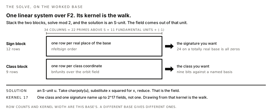
Signature and class are the two halves of one right-hand side. Everything else on this page is how to build those rows correctly.

An aim is a job rather than a lookup: submitting returns a job id, and the output object below is what the finished job holds when you fetch it, not what the submit call returns. Class and unit data from bnfinit is conditional on the generalized Riemann hypothesis unless bnfcertify is run, and we did not run it.

Aim

base_coeffs

Monic irreducible degree-12 base as an integer coefficient list, constant term first. That is Polrev order, and it is the order every polynomial in this contract uses.

s_primes

The rational primes that generate the S-unit group you want to use.

orbit_field

The relation, named rather than guessed. Same coefficient order as the base.

orbit_embedding

The image of the orbit field's generator as an element of the base. Required whenever nfisincl finds more than one embedding. Two embeddings are two different relative-norm maps.

signatures

The real-root counts you want upstairs.

class_element

An element of the orbit field naming the one class you want. Overrides class whenever both are sent. Prefer this form.

class

One of three forms: the mode word twisted for every nonzero reachable class, the mode word squares for the zero class, or an explicit class bound to a prepared basis.

prepared

A handle a previous call returned. Stands in for base_coeffs and s_primes and reuses that preparation's basis.

walk

How many extra fields to draw from the solve's kernel at each class and signature it lands on.

Give a degree instead of a polynomial and you get one result per embedding, not per subfield. A base with no subfield at that degree comes back with nothing to aim rather than a default.

{
  "base_coeffs": [-4337, -14388, 3142, ...],
  "s_primes": [17, 41, 4001],
  "signatures": [24, 16],
  "class_element": [10031, 3653, -25, 8371],
  "orbit_field": [4337, 2685, -160, 1],
  "orbit_embedding": {
    "numerators": [27043677307972, 97447781089076, -40953355656028, -273257184269168,
                   705231691117, 125194392871944, 7641596303894, -18381647173824,
                   -1148991623988, 1036281514444, 38513825866, -19875914124],
    "denominator": 1010521154671
  },
  "walk": 64
}

Both element fields are numerators in Polrev order over one common denominator, and they live in different fields, so their lengths differ. class_element is an element of the orbit field, so it is that field's degree many coefficients, three here, written as the flat list above with the denominator last. orbit_embedding is an element of the base, so it is twelve coefficients in the base's power basis with the denominator named separately; trailing zeros are written, not dropped. The values above are the worked base's, measured. Substituting the embedding into the cubic reduces to zero modulo the base polynomial.

class_element is the safe way to name one class. orbit_embedding may be omitted on the worked base, where nfisincl finds exactly one. The example omits class because class_element is present; sending both is legal and the element wins.

A raw bit string in class is the one input that cannot be validated, so it is not accepted alone. Send it as {"bits": "010000100", "prepared": "<the prepare id a previous call returned>"} and it is checked against that preparation's basis fingerprint and refused if the fingerprint has moved. A bare string is refused with the fingerprint that would have been needed.

{
  "prepared": "12t11-17.41.4001-4a91c0",
  "basis_fingerprint": "sha256:9f2c...",
  "orbit_embedding": {
    "numerators": [27043677307972, 97447781089076, -40953355656028, -273257184269168,
                   705231691117, 125194392871944, 7641596303894, -18381647173824,
                   -1148991623988, 1036281514444, 38513825866, -19875914124],
    "denominator": 1010521154671
  },
  "polynomials": [
    {
      "coeffs": [1, 0, -4, ...],
      "label": "24T10301",
      "label_candidates": [],
      "label_margin": 236.27,
      "signature": 24,
      "class": "010000100"
    }
  ],
  "reachable_classes": ["010000100", "100010000", "..."],
  "unreachable": false
}

Output: polynomials, each carrying its coeffs in the same Polrev order, a signature, the class as a bit string together with the basis_fingerprint that gives it meaning, and the label, which is not solved for but read from the finished polynomial and left null when that route refuses on a thin margin. When the wanted class is not reachable at that S, unreachable is true alongside reachable_classes. Unreachable is never a verdict on the base. Every class string in that output is written against basis_fingerprint, and prepared is the handle to send back.

label is null whenever the reader refuses. label_candidates carries the tied block when the refusal is a tie, and is empty when the refusal is a thin margin. More primes narrow a thin margin and never break a tie. label_margin carries the nats either way, and reads zero inside a tie.

Reach, kernel, and what a class does not fix

Measured on the worked base, the class block runs 7 of 7 at the pair 17 and 4001 and 10 of 16 at seven primes, so widening S raises the reachable count while lowering the share. A signature below 24 does not name one right-hand side: negative at k real places can be asked for in as many ways as there are k-subsets of the places, and those need not agree on the label, so the compiler enumerates them. Reachability belongs to the stacked system rather than to either block.

A class narrows the label rather than fixing it. Calibrating a base means building many fields per reachable class: on the worked base, 200 fields at signature 24 in a single class returned three different groups, 176, 21 and 3. The solve leaves a kernel, 17 wide there, so a class and a signature name up to 2¹⁷ fields rather than one, an upper bound because a solution whose element is already a square in the base adjoins nothing and is skipped. Reducibility of the x² substitution is not that test. An element sitting in a proper subfield still gives a perfectly good degree-24 field, and that is exactly the imprimitive case the walk exists to find. Step 6 of the by-hand recipe below keeps the two tests apart. Classes do not carry across bases. The 6×4 table is the exception: there the label is a function of (a, b, ε) before any field is built.

What one aim costs, measured

On the worked base, bnfinit is 38 to 43 milliseconds across three runs, decomposing the three rational primes into the 22 primes above them is one or two more, and bnfunits over those 22 is 12, so preparing the base from nothing is about 55. Prepare a base once and every later aim on it skips that: send the prepared handle the first call returned instead of base_coeffs and s_primes. The response carries the same basis_fingerprint or the call is refused.

Building one degree-24 polynomial is about 16 milliseconds, essentially all of it polredbest. Labelling is about 110 milliseconds a field after a one-time third of a second to load the cycle-type table. The whole published file runs in 0.86 seconds. An aim is dominated by per-field work, roughly 130 milliseconds of it. One aim's field count is the number of right-hand sides times walk plus one. The example above asks for signature 24 (one right-hand side) and signature 16 (495 of them on a totally real degree-12 base), with 64 extra fields at each: 496 times 65 is 32,240 fields. A pair that comes back unreachable costs a solve instead of a field. Total work depends primarily on the number of fields requested; these timings describe the worked base.

By hand

On a quadratic-step base you already have, this is the method to run directly in PARI.

1. bnfinit the degree-12 field and its small subfields, not the closure.
2. idealprimedec on the base at each of your S-primes, then bnfunits on that list of prime ideals, not bnfsunit and not the rational primes. bnfsunit hands back the prime generators alone, 22 on the worked base. bnfunits hands back all 34: those 22 plus the 11 fundamental units plus −1. That vector, in the order it returns it, is the unknown. Expand each generator with nffactorback before anything arithmetic touches it.
3. bnfinit the orbit field F. Take the primes of F above your S-primes with idealprimedec, and call bnfunits(F, those). The length of its first component is the class width. Give F a variable of lower priority than the base's, F in y against the base's x.
4. Factor the base over F with nffactor and keep the factor of degree 12 over the degree of F, four in the worked case, that vanishes on the embedding. For each expanded base S-unit g, polresultant(rel, g, x) is its relative norm and bnfisunit(F, that, UF) gives the exponent vector; mod 2 that is g's column of the class block.
5. The sign block is built the same way, one column per basis unit and one row per real place of the base, in the order nfeltsign returns them. On a totally real base, signature 24 is the all-zero right-hand side. Stack the blocks. On the worked base that is twelve sign rows above nine class rows, 21 by 34. Solve with matsolvemod on the stacked matrix and right-hand side reduced mod 2. The walk basis is matker of Mod(stacked, 2), 17 vectors wide here.
6. The solution is an S-unit u. Take charpoly of u over the base, substitute x² for x, then polredbest. First check that u is not already a square in the base and that it generates the base rather than a proper subfield, because charpoly is the minimal polynomial only when u generates the base.

All of this is the block case, where F lies inside the base. A relation that is not a block has its orbit field built from the roots, and that case is not exhibited here. Do not copy a class from another base, and do not copy a bit string between runs even on the same base. Name a class by an element of F and read your coordinates off it with lift(bnfisunit(F, w, UF)) % 2. The class calibrated here is w = (−25y^2 + 3653y + 10031)/8371 in F = Q[y]/(y^3 − 160y^2 + 2685y + 4337), which reads 010000100 on PARI 2.13.3. An element is attached to a model of F, to one embedding of F into the base, and to S: transport it across a different model with nfisisom, count embeddings with nfisincl (1 on the worked base), and check it is an S-unit at your S before trusting a coordinate read from it.

Label

PARI will not do this for you. polgalois stops at degree 11. Magma's GaloisGroup handles degree 24 and returns a certificate rather than a statistic, so use it if you have it. Otherwise read the label statistically. The first four steps determine the output. The accept rule is a hard threshold, so a margin sitting within float error of 5 nats could be accepted by one implementation and refused by another; the thinnest we have measured at 1,000 primes is 19 nats. The fifth step is what that method scored when we tested it, not a step. The group table in step 1 is a cache you either build or ask for.

1. The group side, computed once and reusable forever. For each candidate group, take its conjugacy classes, and for each class the cycle type of its elements acting on the 24 points, weighted by class size over group order. That is a probability distribution over cycle types, one per group. GAP's transitive groups library supplies the candidates as TransitiveGroup(24, n). Ours came to 41 MB across the 25,000 groups of degree 24. We never timed the GAP run that produced it. Build your own or write and we will send ours.
2. The field side. Normalize to a primitive integer polynomial with positive leading coefficient, then walk the primes in increasing order starting at 3 and stop once you have admitted a thousand, with an upper cap of 5×10⁷. Deterministic, no sampling. Skip any prime dividing the leading coefficient. Admit a prime exactly when the factorization modulo it is squarefree and its factor degrees still total 24. The multiset of factor degrees at an admitted prime is the cycle type of a Frobenius element on the roots, and Chebotarev says those types arrive at exactly the frequencies in step 1.
3. Score. For each group, sum count × log rate over the observed types, where rate is that group's probability for that type. A group that assigns probability zero to a type you actually observed is excluded outright rather than scored low. Take the highest total.
4. Accept or refuse. The margin is the winner's total minus the runner-up's, in nats. Accept at 5 nats or more and refuse below that, reporting the field as unlabelled rather than guessing. Two groups whose cycle-type distributions are equal are inseparable at any number of primes, so when the top of the list is a tie the honest output is that short list, not a name. If the exclusion rule in step 3 empties the candidate list, do not widen the rule: report zero surviving candidates.
5. What this was measured against. On 100 fields the organizer had already labelled, it returned 100 correct with every winner ahead by at least 19 nats. Fed shape data planted from a deliberately wrong group it returns that wrong group, 77 of 77. It separates all 87 pairs in our set that share a base group but carry different labels. At 1,000 primes every gate row cleared 19 nats; at 300 primes all rows were still correct but one came down to 0.76. The thinnest margin among the nine fields of the worked instance was 229.9 nats, the widest 276.2. Reading all nine took 1.30 seconds, one alone 0.44, so the cycle-type table loads in about a third of a second and each field costs about 0.11 after that.

Either way the label is read after the build, never before, and it is the label that turns your field into a cell.

Predict a 6×4 label

Input: family, which is 6x4 and selects this table rather than an aim; a and b, the exponents in the ideal ((x−1)^a(x+1)^b) of 𝔽₃[x]/(x⁶−1) with 0 ≤ a, b ≤ 3; and epsilon, written ε in the classification, which records whether the twist vanishes. Sixteen ideals times two twist states is 32 triples, and 24 of them are admissible. Output: the 24T label and the group order. This is a table lookup on a proved classification. All twenty-four rows are printed in the classification.

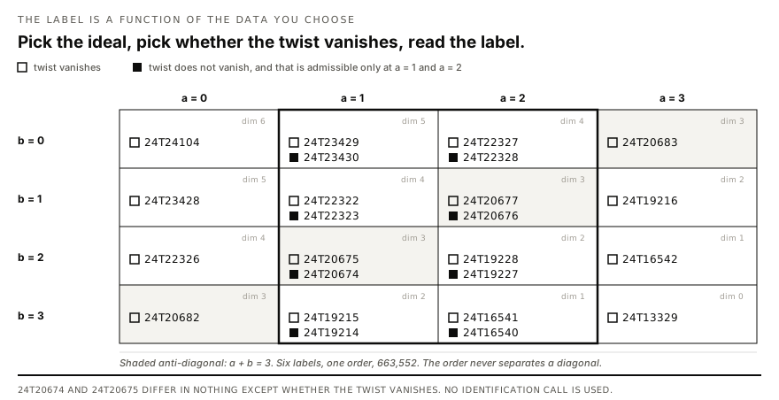
The lookup below is this grid. The request names a square and a twist state, and the reply is the label in it.

{
  "family": "6x4",
  "a": 1,
  "b": 2,
  "epsilon": 0
}

{
  "label": "24T20675",
  "order": 663552
}

What this will not do

It will not submit to the organizer. It will not certify with Magma. It will not invent a construction you do not have. If your recipe never produces a relation the orbit field can see, the compiler has nothing to aim.

The published file stops at polynomials and carries no labelling code. Its nine fields were labelled separately with the reader above: eight 24T10301 and one 24T5392. The host labels what it builds. Write to hello@recognitionphysics.org if the host refuses a job the contract allows.